Coarse Classing by Hand: Reversals and Policy Breaks
By Hafizh Yuwan Fauzan · 2026-10-15
Binning deep dive 3 of 5: coarse classing by hand. Deep dive 2 made the first cut into deciles; this one merges them into the groups a scorecard actually uses.
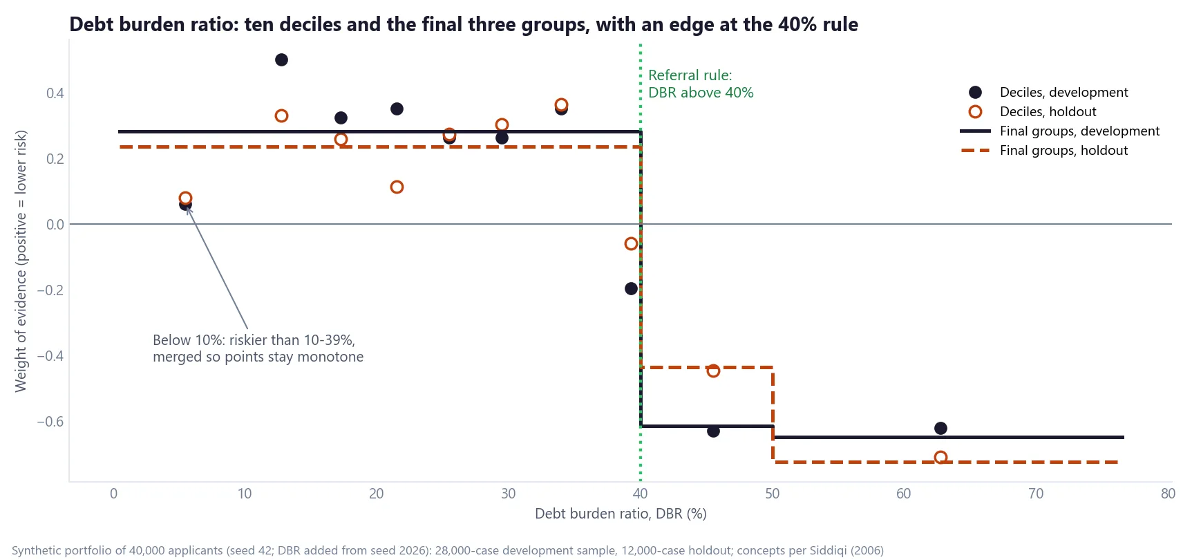
The fictional lender in my synthetic portfolio refers every application with a debt burden ratio (DBR) above 40%, and I built a step in risk at that line into the data. Cut the ratio into deciles, the way I start every characteristic, and one decile runs from 36.5% to 42%. It straddles the rule. Its weight of evidence (WOE) is −0.20 on the development sample and −0.06 on the holdout: half safe, half risky, and different on each sample.
Equal-sized groups don't know the lender has a rule at 40%. Coarse classing is where you tell them. It is the step where fine groups are merged, by hand, into the handful of groups that will each get points, and where business knowledge goes into the scorecard on purpose.
DBR is what Indonesian lenders often call the share of income going to debt repayments; N. Siddiqi's Credit Risk Scorecards (Wiley, 2006) calls it the debt service ratio. All numbers come from the synthetic portfolio of 40,000 applicants used in the credit scorecard series, with DBR added for this series. As before, WOE is the log of a group's share of goods over its share of bads, so positive means lower risk.
What coarse classing does
Siddiqi's standard for a final grouping is that attribute strengths "must also be in a logical order, and make operational sense" (p. 83). Logical doesn't mean straight: he asks for "logical (not necessarily linear)" relationships. Getting there "is one of trial and error" (p. 83), balancing a clean trend against keeping enough information value (IV).
Three kinds of decision come up again and again:
- Where the edges go. Merge neighbouring fine groups whose weights are close, and put an edge where the risk really changes or where the business draws a line.
- What to do with a reversal. A group that breaks the trend is either noise, to be merged away, or real behaviour, to be kept and explained.
- How to group categories. For a characteristic with no order, such as residential status, group values with similar weights that also make business sense.
He also warns that the process "can be abused" by someone "not familiar with the business" (p. 85). Coarse classing is a judgement made with the business, not only an optimisation.
Put the break where the policy is
I always put a group edge at a policy cut-off. Siddiqi makes the same case with this exact characteristic: if loans with a debt service ratio above 42% are referred, the ratio should be "grouped with a break at 42%" (p. 87). That way, he argues, the distortion the policy rule causes in the scorecard is minimised, because the applicants it affects are isolated somewhat. Such groupings can also test the conventional wisdom behind the rule.
Here is what that edge is worth in our data. The first grouping only merges deciles, so its edges sit on decile boundaries (10.5%, 36.5% and 49%); the second uses 10%, 40% and 50%, putting an edge on the policy line:
| Grouping | Groups | IV, development | IV, holdout |
|---|---|---|---|
| Deciles merged, no edge at 40% | <10.5%, 10.5–36.5%, 36.5–49%, 49%+ | 0.154 | 0.124 |
| Edge at the 40% rule | <10%, 10–39%, 40–49%, 50%+ | 0.180 | 0.139 |
| Final, monotone | <40%, 40–49%, 50%+ | 0.175 | 0.135 |
With the same number of groups, moving the edges to the policy line raises IV by about 17% on development and 12% on the holdout. In the merged-decile grouping, the straddling decile is diluted into 36.5–49% (−0.43 on development, −0.27 on the holdout), mixing applicants from both sides of the rule. The 40% edge puts everyone above the rule into their own groups, which are clearly riskier on both samples (40–49% at −0.62 and −0.44).
The reversal at the low end
The chart shows one more feature. Applicants with a DBR below 10% are riskier than those between 10% and 39%: WOE +0.05 against +0.32 on development, and +0.04 against +0.26 on the holdout. With 239 bads behind it, this isn't the kind of noise deep dive 2 dealt with. It holds in both samples. (I built this into the synthetic data too, to give this section a real decision to make.)
Siddiqi's rule is clear: reversals "should be investigated first", because they "may be reflecting actual behavior" (p. 84). A U shape can stay "as long as the relationship can be explained". His own example is utilisation on revolving credit in North America, which has a "banana-shaped curve": very low utilisation is riskier, then risk falls, then rises again.
My answer for this characteristic is to merge the low end into the 10–39% group and keep the points monotone. From the bureau side, where I work, monotonic is a must for a credit score. Merging costs very little here: IV falls from 0.180 to 0.175 on development and from 0.139 to 0.135 on the holdout. The final grouping, <40%, 40–49% and 50%+, falls on both samples.
Why monotonic is a must for a bureau score
In my experience at the bureau, a score has to move the way a consumer expects: better behaviour, higher score. Equifax describes its NeuroDecision scoring technology in similar terms:
"This monotonicity allows the NDT algorithm to reward positive behaviour." (Equifax Australia, Explainable AI for Credit Scoring, retrieved 15 October 2026)
Siddiqi's argument for logical groupings points the same way: they keep the points sensible, so that "an older person gets higher points than a younger person always" (pp. 85–86).
In Part 3 of the scorecard series I noted that age is often not monotonic in raw data, and WOE binning can carry that shape. For a bureau score, coarse classing is where I smooth it into monotonic points, deliberately.
When two groups look the same
Above the rule, 40–49% and 50%+ have almost the same weight on development: −0.62 and −0.65. The usual move is to merge neighbours with similar weights. The holdout argues otherwise: −0.44 and −0.73. Both groups clear the 5% minimum (14.5% and 9.4% of cases), and keeping them apart doesn't break the monotone trend on either sample, so the final grouping keeps them separate.
That is a judgement call, and merging them would be defensible too. The point is to make it with both samples on the table, not from the development weights alone.
Grouping a characteristic without an order
Residential status has four values and no natural order. Siddiqi's guidance is to put "attributes with similar WOE together" (p. 84), while also checking regional and operational sense (p. 87). His example is mortgages, where postal codes should be grouped by similar real-estate markets rather than by state.
| Residential status | Share | WOE, development | WOE, holdout |
|---|---|---|---|
| Own | 42.3% | +0.39 | +0.40 |
| Rent | 35.9% | −0.19 | −0.25 |
| With parents | 14.8% | −0.31 | −0.28 |
| Other | 7.0% | −0.22 | −0.04 |
Almost all the information is in one split. "Own versus everything else" keeps an IV of 0.086 against 0.087 for all four groups. "Other" is the unstable one: −0.22 on development, −0.04 on the holdout, from 237 bads. Merging it into "Rent", the value its development weight is closest to, gives three groups (own, rent or other, with parents) with an IV of 0.087 and no unstable group.
Whether to keep "With parents" separate is the business question. It looks slightly riskier than renting on both samples (−0.31 and −0.28 against −0.19 and −0.25), and it clears the 5% minimum at 14.8%. Statistics alone can't settle whether that difference is worth a separate group of points; the people who know the product can.
A checklist for coarse classing
- Start from the fine groups and a stable view of them: development and holdout side by side.
- List every policy cut-off that applies to the characteristic and put a group edge exactly on each.
- Merge neighbours whose weights are close on both samples, not just one.
- For each reversal, check the bad count and the holdout, then decide: merge it or explain it.
- For a bureau score, make the final points monotonic. Elsewhere, keep a reversal only if you can explain it and the reason codes still make sense.
- Check every final group against the 5% minimum.
- Group categories by similar weights and by business meaning; merge small unstable values into their nearest neighbour.
- Record each decision and its reason. Coarse classing is where most of a scorecard's judgement lives.
Next in this series: WOE-based binning by algorithm, and how its answer compares with the groups chosen by hand here.
If you handle reversals or policy breaks differently, I would like to hear how. Get in touch.
Hafizh Yuwan Fauzan (Hafizh Fauzan) is a credit risk data scientist in Jakarta, Indonesia, building scorecards and machine learning models on national-scale credit data.