Fine Classing in Credit Scorecards: How Many Groups to Start With
By Hafizh Yuwan Fauzan · 2026-10-14
Binning deep dive 2 of 5: fine classing. Deep dive 1 dealt with missing values and outliers; this one makes the first cut.
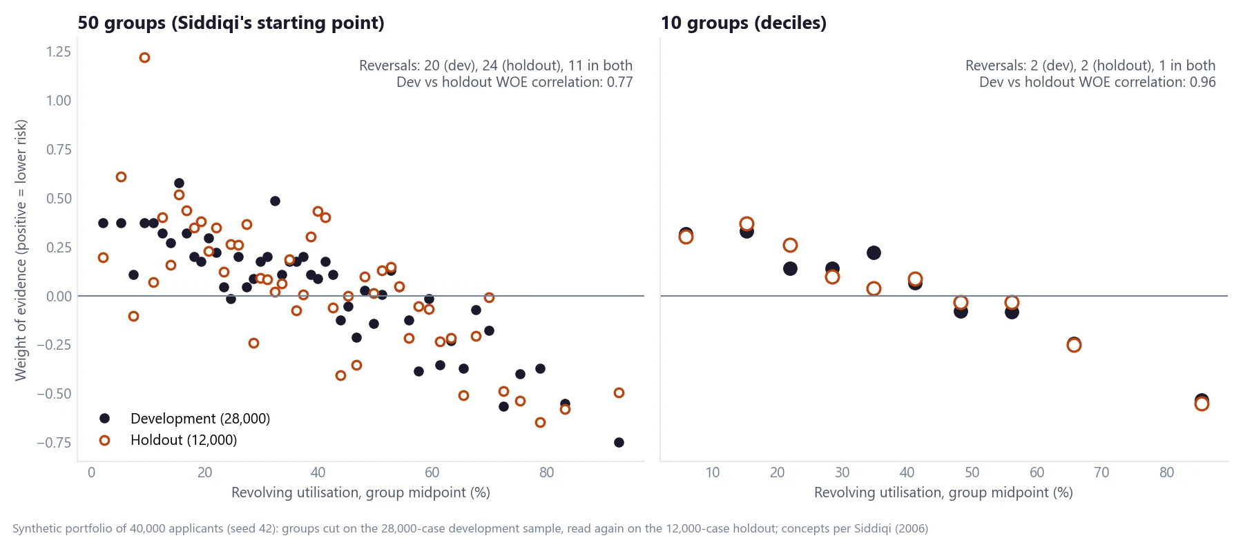
I built the utilisation characteristic in my synthetic portfolio as a straight line: the more of their credit limit applicants use, the riskier they are, with no bumps. For this test I cut it into 50 equal-sized groups, the starting point N. Siddiqi suggests in Credit Risk Scorecards (Wiley, 2006). Read group by group, the weight of evidence (WOE) goes the wrong way 20 times out of 49 steps.
None of those 20 reversals is real. I know, because I wrote the formula. In real data you don't have the formula, and that is the whole problem fine classing has to solve: cut fine enough to see the shape, without mistaking noise for shape.
All numbers come from the synthetic portfolio of 40,000 applicants used across the credit scorecard series. Groups are cut on the 28,000-case development sample and read again on the 12,000-case holdout. As in Part 3 of the scorecard series, on WOE and IV, WOE is the log of a group's share of goods over its share of bads, so positive means lower risk.
What fine classing is
Fine classing is the first, deliberately detailed grouping of a characteristic, before any groups are merged. Siddiqi never uses the term. He calls the whole step grouping, part of what he names initial characteristic analysis (pp. 77–87), but his recipe is what the industry calls fine classing:
- For a numeric characteristic, start with "50 or so equal groups" (p. 79). Oddly, his sentence says "nominal variables", but the advice only makes sense for numbers you can sort.
- For a categorical characteristic, calculate "the WOE for each unique attribute" (p. 79), so every value starts as its own group.
- Decision trees can suggest cut points too, though he notes that "most users, however, use them to generate initial ideas" and then fine-tune by hand (p. 79).
The output isn't a scorecard group yet. It is a picture of the relationship between the characteristic and risk, detailed enough to show its shape. The next step, coarse classing, merges those fine groups into the final ones.
Fifty groups or ten
I don't start with 50. I start with deciles: ten groups, using pandas qcut in Python. Ten is only the initial cut anyway. Here is what each choice shows on the same characteristic.
| Groups | Reversals, development | Reversals, holdout | Reversals in both | WOE correlation, development vs holdout |
|---|---|---|---|---|
| 50 | 20 of 49 steps | 24 | 11 | 0.77 |
| 20 | 7 of 19 | 8 | 4 | 0.91 |
| 10 | 2 of 9 | 2 | 1 | 0.96 |
With 50 groups, each group holds 560 development cases and between 33 and 107 bads. That sounds like plenty, but a WOE built on 40 bads moves a lot when a few of them land one group over. The deciles hold about 2,800 cases each, and their weights barely move between development and holdout.
Fifty groups aren't wrong. They show more detail, and if the relationship had a real kink at 40% utilisation, 50 groups would show it sooner than ten. The cost is that you then have to sort the real kinks from the 20 fake ones. Starting from deciles trades a little resolution for far less noise to argue with.
Telling noise from a real pattern
I judge a reversal on two things: stability and a business explanation. A real pattern shows up in every sample you look at; noise moves. When a fine-classed WOE reverses, I compare it across every snapshot I have and the out-of-time sample, and ask whether the reversal is still there.
The chart is the gentlest version of that test. The holdout is a random 30% of the same applicants, not a later period. Even so, only 11 of the 50-group reversals appear in both samples. If the two sets of reversals were completely unrelated, you would expect about 10 to coincide by chance (20 × 24 / 49). Noise that fails a random holdout will almost certainly fail an out-of-time sample too.
The other test is a business explanation. Siddiqi allows a reversal or a U-shape to stay if experience can explain it (pp. 83–84), and that is the next article's subject. A reversal needs both: a reason it should exist, and evidence that it does in every sample. As a set, the 20 reversals here have neither: no reason to exist, and no more overlap with the holdout than chance.
Small samples make noise look like strength
Noise doesn't only bend the trend. It also inflates information value (IV), the measure used to rank characteristics. Here is the same characteristic's IV at each number of groups, on the development sample, the holdout, and a random draw of about 10% of the development sample (2,781 cases):
| Groups | IV, development (28,000) | IV, holdout (12,000) | IV, 10% sample (2,781) |
|---|---|---|---|
| 50 | 0.085 | 0.114 | 0.212 |
| 20 | 0.075 | 0.082 | 0.137 |
| 10 | 0.070 | 0.072 | 0.104 |
| 6 final groups (scorecard series Part 3) | 0.064 | – | – |
The relationship is identical in every row. Yet on the small sample, 50 groups report an IV of 0.21, which Siddiqi's rule of thumb (p. 81) would call medium strength, three times the 0.070 the deciles find on the full data. Even the full holdout crosses into medium at 50 groups (0.114). One of the 50 small-sample groups holds a single bad.
The lesson for fine classing: never rank characteristics by an IV calculated on fine groups, and be most suspicious of fine-classed IV on small samples. Deep dive 5 covers IV properly.
The checks before you move on
Siddiqi lists what a well-grouped characteristic looks like (p. 80). Two of his checks belong at the fine-classing stage:
- A "minimum 5% in each bucket" rule. Deciles pass it by construction, at 10% each. Fifty groups never can, at 2% each, which is fine for a first look but not for a final group.
- No groups with zero goods or zero bads. A group with no bads has no finite WOE at all. On large samples this rarely bites, but the 10% sample was already down to one bad in a group.
A practical warning if you use qcut as I do: when a characteristic has many tied values (months at address with lots of zeros, number of inquiries), the decile edges repeat. pandas then refuses with "Bin edges must be unique", and with duplicates="drop" it quietly gives you fewer groups than you asked for (pandas qcut documentation; checked on pandas 2.3.3, October 2026). Count the groups you got, not the groups you requested.
What equal-sized groups can't see
Equal-sized groups follow where the applicants are, not where the risk changes. In our data, 243 development applicants (0.9%) use 90% or more of their limit, with a WOE of −0.87. The top decile starts at 71% utilisation, so they disappear into it, and the decile's WOE is only −0.53. Even the highest of the 50 fine groups starts at 86%.
Siddiqi's answer is to add breaks where the business knows something happens, such as a policy cut-off (p. 87). That is coarse classing's job, and it's where a fine-classed picture and business knowledge meet. Fine classing should still make the thin tail visible: look at a separate tail cut before you decide it doesn't matter. Part 3 of the scorecard series kept 90%+ as its own group at 0.9% of cases, below the 5% rule; whether a business break justifies that is the next article's question.
A checklist for your first cut
- Recode missing values and special codes first (deep dive 1), so they don't land inside numeric groups.
- Cut numeric characteristics into equal-sized groups: deciles are a sound start, 50 groups if the sample is large and you want detail.
- Give each category of a categorical characteristic its own group.
- Count the groups you actually got after tied values were merged.
- Read the shape, not individual weights. Mark every reversal.
- Check each reversal in the holdout, other snapshots and the out-of-time sample. Keep it only if it is stable and explainable.
- Look separately at thin tails that equal-sized groups hide.
- Don't rank characteristics by fine-classed IV.
Next in this series: coarse classing by hand, where the fine groups are merged into a logical trend and business breaks, such as a referral rule on the debt service ratio, are put in on purpose.
If you start with a different number of groups, I would like to hear why. Get in touch.
Hafizh Yuwan Fauzan (Hafizh Fauzan) is a credit risk data scientist in Jakarta, Indonesia, building scorecards and machine learning models on national-scale credit data.