Missing Values in Credit Scorecards: Why Missing Is an Answer
By Hafizh Yuwan Fauzan · 2026-10-13
Binning deep dive 1 of 5: missing values and outliers. A new series that takes one step of scorecard binning at a time, following N. Siddiqi's Credit Risk Scorecards (Wiley, 2006).
I agree with the rule that every group in a scorecard characteristic should hold at least 5% of cases. Yet in the example below I keep a group holding 3.8%, and I would do the same in any scorecard I build. The group is "Missing", and it is the one group where breaking the 5% rule makes sense.
Siddiqi's own worked example does the same thing. On one page he applies "a general 'minimum 5% in each bucket' rule" and groups Missing separately. His Missing group works out at 2.5% of cases (recomputed from his Exhibit 6.2), and the text never reconciles the two (p. 80). This article is about why the exception holds, and about the treatments that quietly destroy the information Missing carries: dropping, imputing, and special codes nobody documented.
All numbers come from the synthetic portfolio of 40,000 applicants I built for the credit scorecard series, measured on its development sample of 28,000 accounts. Part 3 of that series gave missing values one row in a table. Here they get the whole article.
Missing is rarely random
Time at address is a characteristic most application forms ask for and some applicants skip. In our development sample, 1,062 applicants (3.8%) left it blank. Here is how each group's weight of evidence (WOE) compares. WOE is the log of the share of goods in a group divided by the share of bads, so positive means safer than average and negative means riskier. (Siddiqi multiplies it by 100; I keep the plain log, as in Part 3.)
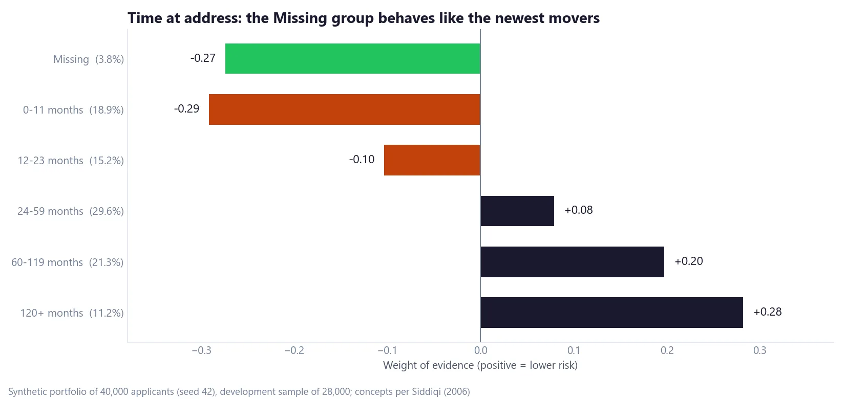
The Missing group's WOE is −0.27 and its bad rate is 12.8%. That is almost exactly the newest movers, who have lived at their address under a year: WOE −0.29, bad rate 13.0%. The development sample as a whole runs at 10.0% (2,813 bads in 28,000).
I built this portfolio, so I know why: the generator makes a blank field riskier. But it mirrors what Siddiqi describes from real data. "Missing values are not usually random," he writes (p. 75). His example is applicants who are new at their job, who are more likely to leave "years at employment" blank. Applicants tend to skip the questions whose honest answer looks bad.
That is the first reason to keep Missing as its own group. Its WOE tells you which real group it resembles, and Siddiqi notes that when Missing's weight sits close to another attribute, "it may shed light on the exact nature of the missing values" (p. 75). Here the light points at recent movers.
Siddiqi's four options
Logistic regression can't take a blank, so something has to happen to every missing value. Siddiqi lists four options (p. 75):
| Option | What it does | The catch |
|---|---|---|
| 1. Drop every record with a missing value | Complete-case analysis | In financial data it leaves very little to work with |
| 2. Drop characteristics or records with many missing values | Siddiqi's example threshold is more than 50% missing | Throws away whatever the blanks were telling you |
| 3. Keep "Missing" as its own group | Missing gets a WOE and points like any other group | Needs enough cases for a stable weight |
| 4. Impute | Fill blanks with a statistical estimate | Assumes the blank holds no information |
His verdict is short: "While the second option may be more convenient, option 3 offers many benefits" (p. 75). He recommends that missing data be assigned points in the final scorecard. That has a practical side as well as a statistical one. Next year, applicants will leave the same field blank, and the scorecard needs a row to score them with.
Options 1, 2 and 4 share an assumption: that a blank means nothing. Siddiqi allows imputation or exclusion only after the missing data has been analysed and found "random and performance-neutral" (pp. 75–76).
In my own work, Missing always gets its own group. I don't impute missing values in a scorecard.
What imputation hides
The most common shortcut is to fill blanks with the average. Siddiqi warns that assigning the mean or most frequent value "will cause spikes in the data" (p. 76). Here is what that looks like in our portfolio.
The mean time at address among applicants who answered is 54.8 months. Fill all 1,062 blanks with it and they land in the 24–59 months group, on a single value. An ordinary single month in that range (54 months) holds 182 applicants, so the spike is nearly six times that. Then:
- The 24–59 group grows from 8,295 to 9,357 cases, and its bad rate rises from 9.4% to 9.7%.
- Its WOE falls from +0.08 to +0.03, so every applicant who really has lived there two to five years now gets fewer points.
- The 1,062 blank applicants, whose bad rate is 12.8%, are scored as if they were a safer-than-average group.
- The characteristic's information value (IV) falls from 0.040 to 0.036. The scorecard has lost information, and nothing flags it.
The median (37 months) does the same damage: it lands in the same group, with 1,310 cases piled on a single value.
Siddiqi adds that the imputed applicants can no longer be told apart from those who genuinely had that value (p. 76). Once the blanks are gone, so is the evidence that they were ever there.
When 0 isn't zero: special codes
Not every missing value arrives as a blank. Siddiqi asks you to check that "0" represents zero and not missing values, and that "special values such as 99 or 999 are documented" (p. 74).
The filler codes I meet most often are 9, 99 and 999. They are dangerous because they look like data. A time at address of 999 months is 83 years: impossible for almost any applicant but not obviously wrong to a model. Left as numbers, they create a fake group of very long-tenured, very stable-looking applicants. They also distort the equal-sized groups you cut at the next step, fine classing (Siddiqi simply calls the whole step grouping).
The fix is the same as for blanks: recode each special value to an explicit label ("Missing", "Not asked", "Refused") before any grouping. Then decide with the data owner whether these are one group or several. Siddiqi even suggests coding blanks on purpose with a value beyond the normal range, such as 99 or 999, so they stay in the analysis (p. 76). Done deliberately and documented, that is the same idea as a label. An undocumented 999 is the opposite: a bug waiting for the next analyst.
Outliers: investigate before you drop
Outliers are the opposite problem: values that are present but outside the normal range. Siddiqi's example is an age distribution running from 18 to 55, with a few applicants at 99, 112 and 134 (p. 76). Most look like keying errors. He notes they are usually excluded, or occasionally set to the mean because there are so few.
His caveat matters more than the treatment: "outliers should be investigated first, since they may point to problems such as fraud" (p. 76). An applicant aged 134 is a keying error. Twenty applicants from one branch with the same unusual income may be something else.
Grouping helps here. Once a characteristic is grouped, an extreme value falls into the top group and gets that group's points, so a single wild number can't pull the whole regression. That is one of the advantages of grouping Siddiqi lists (p. 78). Grouping doesn't do the investigation for you, though. Check the outliers first; then let the groups absorb the genuine ones.
Small Missing groups and the 5% rule
Back to the opening exception. The 5% minimum exists so that every group's WOE rests on enough goods and bads to be stable. The 5% rule is a proxy: what really steadies a weight is the number of bads behind it. Our Missing group has 1,062 applicants and 136 bads, enough for a weight worth reading even at 3.8% of cases.
When Missing is genuinely tiny, a few dozen cases with a handful of bads, its WOE is mostly noise. Some analysts then merge it into the group with the closest WOE, which here would be 0–11 months, the group Missing already resembles. I keep Missing as its own group regardless. A small Missing group just means its WOE deserves less trust, and that is worth stating openly: put its bad count in the scorecard documentation so a reviewer can judge it.
Whether a blank field and a missing bureau record belong in the same group is a different question. An applicant who skips one question on the form is not the same as an applicant with no SLIK credit history at all. In my experience the answer depends on the project, because each project has its own segmentation, a topic I will come back to in a later article (Part 2 of the scorecard series introduces it).
A checklist for your next missing-value review
- Profile every characteristic for blanks, zeros, and codes such as 9, 99 and 999, and get each one documented by the data owner.
- Recode every special value to an explicit label before cutting any groups.
- Compare the bad rate and WOE of Missing with the other groups. If it resembles one, you have learned something about who leaves the field blank.
- Keep Missing as its own group, even below 5% of cases.
- Record how many bads sit behind Missing's WOE, so a reviewer can judge how far to trust it.
- Don't impute unless you have shown the blanks are random and performance-neutral.
- Investigate outliers before you exclude or cap them, and look for clusters, which can signal fraud.
Next in this series: fine classing, the first cut of a characteristic into about 50 equal-sized groups (Siddiqi, p. 79), and what it shows that the final groups hide.
If you handle missing values differently in your scorecards, I would like to hear how. Get in touch.
Hafizh Yuwan Fauzan (Hafizh Fauzan) is a credit risk data scientist in Jakarta, Indonesia, building scorecards and machine learning models on national-scale credit data.