WOE Binning by Algorithm: ChiMerge, Trees and Optimal Binning
By Hafizh Yuwan Fauzan · 2026-10-16
Binning deep dive 4 of 5: binning by algorithm. Deep dive 3 merged deciles by hand; this one asks what an algorithm would have done.
I never let an algorithm propose my bins. I cut deciles with pandas and merge them by hand. So for this article I gave the job to three algorithms instead, on the same debt burden ratio (DBR) I grouped by hand in deep dive 3, and compared what came back.
A decision tree, limited to three groups of at least 5% of applicants each, put its two splits at 9.75% and 39.75%. In this data DBR moves in steps of 0.5%, so 39.75% is exactly the lender's 40% referral rule, found without being told. ChiMerge, started the way its 1992 paper describes and run at the .90 level with no cap on the number of groups, returned 16 groups. Thirteen of them hold less than 5% of applicants, and one holds 15 applicants and not a single bad.
Both results are useful, and neither is a scorecard yet. All numbers come from the synthetic portfolio of 40,000 applicants used throughout this series: groups are fitted on the 28,000-case development sample and checked on the 12,000-case holdout. As before, weight of evidence (WOE) is the log of a group's share of goods over its share of bads, so positive means lower risk.
Three ways an algorithm bins
ChiMerge (R. Kerber, AAAI-92) works bottom up. It starts with every distinct value in its own interval, then repeatedly merges the "pair of adjacent intervals with the lowest" chi-square value, stopping when every remaining pair's chi-square exceeds the threshold (p. 124). Kerber recommends the threshold at "the .90, .95, or .99 significance level", with a cap of "around 10 or 15" intervals (p. 125).
A decision tree works top down, splitting wherever good and bad separate best. Siddiqi mentions trees for grouping in Credit Risk Scorecards (p. 79), and notes that "most users, however, use them to generate initial ideas" before fine-tuning by hand.
Optimal binning treats grouping as an optimisation with constraints. G. Navas-Palencia's formulation (arXiv, 2020) is implemented in the open-source Python library OptBinning. Its documentation lets you require a monotonic trend (monotonic_trend) and a minimum share per bin (min_bin_size), and it starts from a tree's split points by default. I ran version 1.0.0 with both: a rising bad rate and at least 5% per bin.
ChiMerge: different isn't the same as usable
ChiMerge does exactly what it promises. Every pair of neighbouring groups it leaves behind passes Kerber's chi-square test at the .90 level. It even found the policy line, as a tiny group from 39.5% to 40%. Its information value (IV) is the highest of any method here, 0.197 on development and 0.151 on the holdout (leaving out the zero-bad group below, whose WOE is undefined).
But it has no idea what a scorecard group needs. Thirteen of its 16 groups are under the 5% minimum. The top group, 72% and above, has 15 applicants and no bads, so its WOE is undefined. Neighbours flip back and forth: 45.5–46% sits at −1.07 while 46–47% is −0.38. At Kerber's strictest setting, the .99 level, it still leaves six groups, two of them under 1%.
None of this is a flaw in ChiMerge. Kerber designed it to turn numeric attributes into discrete ones for classification algorithms, not to produce groups that each get points. A higher IV from more, smaller groups is the same effect deep dive 2 showed with fine classing.
A tree with a floor finds the rule
The decision tree needed two settings: three leaves and a minimum leaf of 5%. It split at 9.75% and 39.75%, giving groups of 8.9%, 67.2% and 23.9%. Its 40% edge is exactly mine; the difference is at the low end, where I merged below 10% into the main group, and at the top, where I split again at 50%. Its IV is 0.180 on development and 0.132 on the holdout, against 0.175 and 0.135 by hand.
What it keeps is the low-end reversal: below 10% is riskier than 10–39% (WOE +0.05 against +0.32). Deep dive 3 merged that group, because from the bureau side monotonic points are a must. A tree has no notion of that rule unless you add it.
Optimal binning with constraints
OptBinning lets you add the rule. With a rising bad rate required and 5% bins, it returned four groups with splits at 34.75%, 39.75% and 54.25%. On the development sample its weights fall steadily: +0.30, +0.16, −0.61, −0.70. It merged the low-end reversal away, as I did by hand, found the 40% line, and has the best holdout IV of the constrained methods at 0.141.
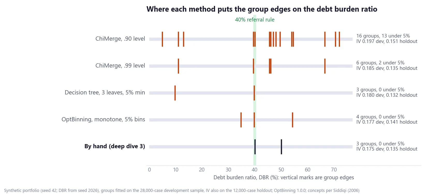
There is one catch, and it is the important one. The 34.75–39.75% group it created is monotone on the data it was fitted on, but not on the holdout. There it sits at +0.29, above the +0.23 of the group below it. The constraint holds where the optimiser could see; nothing guarantees it on new applicants. The hand grouping has no edge between 35% and 40%, and it is monotone on both samples.
Regions: the algorithm does what I do
For a characteristic without an order, the comparison changes. I group regions by risk, merging provinces whose weights are close wherever they are on the map. That is what ChiMerge does when the regions are sorted by bad rate first (an adaptation: Kerber wrote it for numeric attributes). Note that the regional risk pattern in this synthetic data is invented and says nothing about real provinces.
At the .95 level, ChiMerge turned ten regions into four groups:
| Group | Share | WOE, development | WOE, holdout |
|---|---|---|---|
| DKI Jakarta, Bali, Central Java | 34.2% | +0.20 | +0.26 |
| Banten, South Sulawesi, East Java, East Kalimantan | 33.9% | +0.03 | −0.06 |
| West Java | 20.3% | −0.11 | −0.16 |
| North Sumatra, Papua and Maluku | 11.6% | −0.38 | −0.23 |
Every group clears 5%, which the ten single regions don't (three are under it), and the order holds on the holdout. On development, IV barely moves: 0.036 against 0.038 for all ten regions. On the holdout the ten single regions score higher, 0.050 against 0.034, from groups that include those three small ones. OptBinning kept seven groups, including Banten on its own, which flips from +0.06 on development to −0.23 on the holdout.
Siddiqi adds a second test for this kind of grouping: regional and operational sense, such as grouping postal codes for a mortgage scorecard by similar real-estate markets (p. 87). Grouping North Sumatra with Papua and Maluku passes the risk test. Whether it passes the business one is a question for the people who run those regions.
What the comparison shows
On this data the algorithms found the real signal. The tree and OptBinning both put an edge on the 40% rule without being told about it. What they needed from an analyst was everything around the signal: a minimum group size, a monotonic trend, and a check on a second sample. ChiMerge without a size floor produced groups no scorecard could use. The tree kept a reversal a bureau score can't have. OptBinning satisfied its constraints on the development data and broke one on the holdout.
My own practice stays the same: deciles, then merging by hand. If you do use an algorithm, Siddiqi's description of how most users treat trees, "to generate initial ideas", is the right job for it.
A checklist if you bin by algorithm
- Set a minimum group size (5%) before anything else; ChiMerge has none by default.
- Require the trend you need, such as monotonic for a bureau score, rather than fixing it afterwards.
- Read the result on a holdout or out-of-time sample. Constraints are only guaranteed on the data the algorithm saw.
- Move edges that land next to a policy cut-off onto the cut-off itself.
- For categories, sort by bad rate before merging neighbours, then check that the groups make business sense.
- Don't choose between methods by development IV alone. Splitting a group never lowers it, so finer groupings tend to win.
- Record which algorithm, which settings and which version produced the groups.
Next in this series: information value itself, what it measures, why splitting a group never lowers it, and when a very high value should worry you.
If you let an algorithm propose your bins, I would like to know which one and why. Get in touch.
Hafizh Yuwan Fauzan (Hafizh Fauzan) is a credit risk data scientist in Jakarta, Indonesia, building scorecards and machine learning models on national-scale credit data.