Population Stability Index (PSI) in Depth: Bands, Noise and Thresholds
By Hafizh Yuwan Fauzan · 2026-10-20
Stability deep dive 1 of 5: the population stability index. The scorecard series ended with monitoring after go-live; this series takes each stability check apart, one at a time.
Eighteen months after go-live, I calculated the population stability index (PSI) for one month of applicants three times. Against development deciles it was 0.170. Against 20 equal-sized groups it was 0.180. Against fixed 20-point score bands it was 0.166. Same applicants, same scorecard, same development sample.
None of the three is wrong. PSI is not a property of the population alone: it also depends on how you cut the score, how many applicants you have and what you do with an empty band. This deep dive is about those choices, and about where the familiar 0.10 and 0.25 lines come from.
Part 7 of the scorecard series introduced PSI with one worked example. The numbers here come from a new, separate simulation: 36 monthly cohorts of 2,000 applicants (this article uses the first 19) for the same fictional lender after it went live at a 540 cutoff, scored with the scorecard from Part 5 and compared with its 28,000-account development sample. Because it is a separate simulation, its figures don't match Part 7's.
The formula, and one property worth knowing
PSI compares the share of applicants in each score band now (actual) with the share at development (expected), for example 18.6% against 9.4% in the lowest band below:
PSI = Σ ( actual − expected ) × ln( actual ÷ expected ) (over score bands)
The shares go in as proportions (0.186, not 18.6), otherwise the result comes out 100 times too big. Every band adds a non-negative amount, so PSI only grows as distributions move apart. It is also symmetric: swap development and recent applicants and you get the same number. That is because PSI is the sum of the two Kullback–Leibler divergences, one in each direction. In practice it means PSI tells you how far the population moved, not in which direction. The direction comes from the band table.
Bands: why I use development deciles
My choice is development deciles, the same starting cut I use for binning and information value: cut the development scores into ten groups of 10% each, then count recent applicants in the same bands. Here is month 18:
| Score band | Development | Month 18 | Contribution |
|---|---|---|---|
| Below 525 | 9.4% | 18.6% | 0.063 |
| 525–536 | 10.1% | 15.0% | 0.020 |
| 537–544 | 9.5% | 11.4% | 0.003 |
| 545–551 | 9.4% | 10.5% | 0.001 |
| 552–558 | 11.0% | 10.4% | 0.000 |
| 559–565 | 10.2% | 9.1% | 0.001 |
| 566–572 | 9.5% | 6.3% | 0.013 |
| 573–580 | 10.2% | 7.4% | 0.009 |
| 581–591 | 9.8% | 6.0% | 0.019 |
| 592 and above | 10.9% | 5.2% | 0.041 |
| PSI | 0.170 |
Scorecard points are whole numbers, so the "deciles" hold 9.4% to 11.0% rather than exactly 10%. The story is in the two ends: twice as many applicants below 525, half as many at 592 and above. The middle bands barely contribute.
Deciles have two advantages. Every band starts with enough applicants, so no single thin band can dominate the index. And the bands are fixed once, at development, so every month is compared on the same grid.
Fixed score bands (500–519, 520–539 and so on) are easier to explain to a credit committee, because they line up with the cutoff and the strategy bands. Their weakness is the tails. In this portfolio the 620–639 band holds 0.6% of development and the 640+ band none at all. A band that thin can swing on a handful of applicants, and an empty one needs the fix in the next section.
Twenty equal-sized groups give a finer picture, but each band then holds 5%, and the index picks up more noise (next section). The three numbers in the opening differ by 0.014, small next to the shift itself, but large enough to put two of them either side of a line if the month had been closer to one.
So choose one banding, write it down, and never compare a PSI on one banding with a PSI on another.
Empty bands, and the small-number fix
The formula divides by the expected share and takes a logarithm of the ratio. If a band is empty in either sample, one of those is undefined.
It happens more than you would think. Cutting the same quiet month (month 1) into 5-point bands gives 42 bands, and 9 of them are empty that month. The usual fix is a floor: replace any zero share with a small number before calculating. I use 0.0001, which is what the tables here use.
The floor keeps the calculation alive, but the result is not comparable with a PSI on other bands. In month 1, with nothing happening, the 5-point bands gave a PSI of 0.016 against 0.006 on deciles: the extra came from noise, not from any shift. If you see many empty bands, the bands are too fine for the sample, and the fix is wider bands, not a better floor.
How big is zero?
A PSI is never exactly zero, even when nothing has changed. Two samples drawn from the same population differ by chance, and PSI counts that difference as shift.
For a sample this size there is a rough no-change level:
No-change PSI ≈ ( number of bands − 1 ) × ( 1 ÷ recent applicants + 1 ÷ development applicants )
With ten bands, 2,000 applicants a month and 28,000 at development, that is 9 × (1 ÷ 2,000 + 1 ÷ 28,000) ≈ 0.005. To check it, I drew 500 months of 2,000 applicants from the development scores themselves, so with no shift at all. Their average PSI was 0.0045, and the highest of the 500 was 0.014. The first three months after go-live, before the applicant mix moved, scored 0.006, 0.009 and 0.004.
That gives a practical noise zone: I treat anything up to three times the no-change level, about 0.015, as noise. If the chi-square result below holds, that is close to a 99.9% critical value for ten bands (0.0149). On a 99% test, a lower bar (0.0116), months 5 and 6 (0.012 each) would already count as a real move.
The no-change level matters most when samples are small. A lender with 500 applicants a month would see about 0.018 with nothing happening. On 5-point bands (42 bands, so 41 × the same bracket) the level rises to about 0.022 even at 2,000 a month, which is why the empty-band example above looked worse.
The yardstick has a statistical basis. A 2023 review by du Pisanie and co-authors summarises work by Yurdakul and Naranjo in the Journal of Risk Model Validation (2020): a rescaled PSI follows a chi-square distribution in large samples, so critical values depend on both sample sizes and the number of bands, and they argue for those critical values instead of fixed thresholds. Dividing PSI by (1 ÷ recent + 1 ÷ development) and comparing it with a chi-square on (bands − 1) degrees of freedom gives the yardstick above: a chi-square's average equals its degrees of freedom, so PSI averages about (bands − 1) × (1 ÷ recent + 1 ÷ development).
Where 0.10 and 0.25 come from
The bands are familiar. Siddiqi's Credit Risk Scorecards (Wiley, 2006) gives them as a rule of thumb: below 0.10, no significant change; 0.10 to 0.25, a small change that needs investigating; above 0.25, a significant shift (p. 137). The same du Pisanie review traces this interpretation to E. M. Lewis's An Introduction to Credit Scoring (1994).
So the lines are decades old, and they were never tied to a sample size or a number of bands. A fixed line can't know that 0.03 is a real move at 28,000 applicants a month and within noise at 500.
In my work, I don't treat 0.10 and 0.25 as fixed lines. What counts as a worrying PSI depends on the scorecard type. I read the number against the scorecard it belongs to, and against its own history, before I read it against a table.
Reading a slow drift
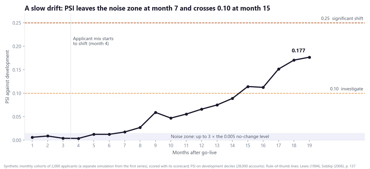
The chart above shows why the history matters. From month 4 the simulated applicants get gradually younger and use more of their credit limits, the same direction of drift as in Part 7. Nothing jumps. PSI leaves the noise zone at month 7, wobbles (month 9 at 0.059, then month 10 at 0.047), crosses 0.10 at month 15 and reaches 0.177 by month 19.
A single month can mislead in either direction: month 16 dips below month 15 even though the drift keeps going. Siddiqi recommends running stability reports on the last three and six months to separate trends from one-month quirks (p. 163), and a three-month average here rises every month from month 5. And by the time the index crosses 0.10, the shift has been building for eleven months, and PSI has been above the noise zone for eight. Watching the trend, not just the threshold, buys time.
PSI tells you that the population moved and how far. It doesn't tell you which characteristics moved or what it costs in points. That is characteristic analysis, the subject of the next deep dive.
PSI on one card
| Formula | Σ (actual − expected) × ln(actual ÷ expected), shares as proportions |
| Bands | Fix them once, at development. I use development deciles. |
| Empty bands | Floor the share at 0.0001; many empty bands mean the bands are too fine |
| No-change level | (bands − 1) × (1 ÷ recent + 1 ÷ development); up to 3 × that is noise |
| Rule of thumb | below 0.10 stable, 0.10–0.25 investigate, above 0.25 significant (Lewis 1994; Siddiqi p. 137) |
| How I read it | Against the scorecard type and its own trend, over three and six months |
If you set PSI thresholds differently for different scorecards, I would like to hear how. Get in touch.
Hafizh Yuwan Fauzan (Hafizh Fauzan) is a credit risk data scientist in Jakarta, Indonesia, building scorecards and machine learning models on national-scale credit data.