Information Value in Credit Scorecards: When to Distrust It
By Hafizh Yuwan Fauzan · 2026-10-19
Binning deep dive 5 of 5: information value. Deep dive 4 compared algorithms with hand-made groups; this one looks at the number used to judge them all.
I generated a characteristic from random numbers, with no connection to whether an applicant later went bad, and cut it into 50 equal-sized groups. On a random 10% of the development sample, 2,781 applicants with 263 bads, its information value (IV) averaged 0.216 over 100 draws. By the rule of thumb in N. Siddiqi's Credit Risk Scorecards (Wiley, 2006), that is a characteristic of medium strength.
IV is the standard way to rank characteristics before building a scorecard, and it deserves that place. But it is a number with habits. It rises when you add groups, it rises when the sample shrinks, and it says nothing about what a characteristic adds next to the others. This last deep dive is about reading it with those habits in mind.
Part 3 of the scorecard series introduced the formula and Siddiqi's bands: below 0.02 unpredictive, 0.02 to 0.1 weak, 0.1 to 0.3 medium, 0.3 and above strong (p. 81). All numbers here come from the same synthetic portfolio of 40,000 applicants, plus three characteristics I added for this series (debt burden ratio, region and worst days past due), generated to behave like their real counterparts. Groups are fitted on the 28,000-case development sample.
What IV adds up
IV is a sum over groups: each group adds the difference between its share of goods and its share of bads, multiplied by its weight of evidence (WOE). A group contributes a lot when it is both large and far from the average.
Worst days past due (DPD) in the last 12 months is the strongest of the characteristics I added, built to look like a bureau DPD variable. Its IV is 0.639; for comparison, Part 3's delinquency count (last 12 months) scores 0.147. Here is where the 0.639 comes from:
| Worst DPD | Share | Bad rate | WOE | IV contribution | Share of IV |
|---|---|---|---|---|---|
| 0 | 66.9% | 5.5% | +0.65 | 0.217 | 34% |
| 1–29 | 13.9% | 10.6% | −0.06 | 0.001 | 0% |
| 30–59 | 8.4% | 17.9% | −0.67 | 0.049 | 8% |
| 60–89 | 4.9% | 24.8% | −1.08 | 0.087 | 14% |
| 90+ | 5.8% | 37.0% | −1.66 | 0.285 | 45% |
Almost four fifths of the IV comes from the two ends: the two thirds of applicants with no delinquency at all, and the 5.8% who reached 90 days. The 1–29 group, at a bad rate close to the 10.0% average, contributes almost nothing (0.001). Reading the contributions tells you which part of a characteristic is doing the work. A small contribution doesn't make a group safe to merge, though: folding 1–29 into 0 would cut IV from 0.639 to 0.581, because their weights (−0.06 and +0.65) are far apart. Merge neighbours whose weights are close.
IV depends on the grouping
The same characteristic has a different IV for every grouping. Splitting a group can never lower IV on the data it is calculated on, as long as every group keeps some goods and bads, so finer groupings usually score higher:
| Characteristic | Final groups | Deciles | 20 groups | 50 groups |
|---|---|---|---|---|
| Utilisation | 0.064 (6 groups) | 0.070 | 0.075 | 0.085 |
| Debt burden ratio | 0.175 (3 groups, deep dive 3) | 0.168 | – | 0.197 |
The relationship between utilisation and risk is identical in every column. Only the cut changed. "Usually" matters: the debt burden ratio's deciles score below its three final groups, because the decile edges miss the 40% policy line that the final groups sit on.
I calculate IV on both: on deciles to screen characteristics, and on the final groups to report them. The two numbers answer different questions, and comparing characteristics only makes sense when they are grouped the same way.
The IV of nothing
The opening example wasn't a fluke. A characteristic with no information at all still gets a positive IV, because sampling noise always makes some groups look a little better or worse than average. How much depends on two things: the number of groups and the number of bads.
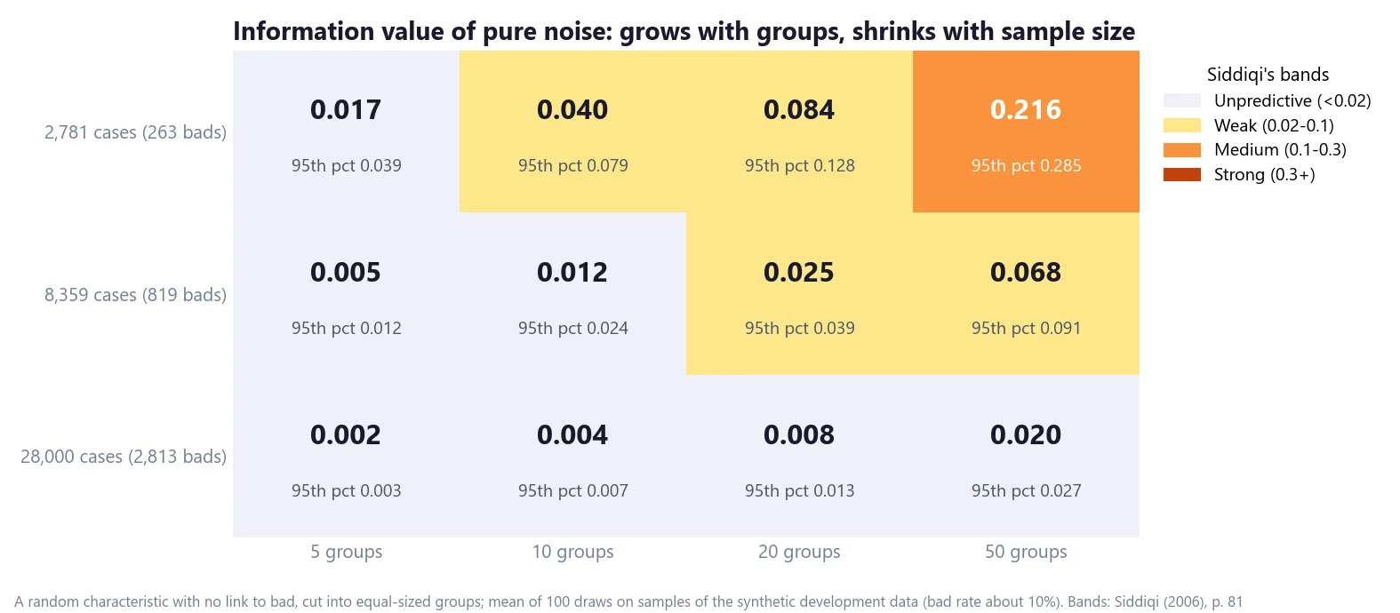
On the full development sample, noise averages about 0.02 even with 50 groups (95th percentile 0.027). On 2,781 cases, with 263 bads, ten groups of noise average 0.040, "weak" rather than unpredictive, and 50 groups average 0.216, "medium".
A useful yardstick matches the simulation closely: the average IV of pure noise is roughly the number of groups minus one, times (1 ÷ number of goods + 1 ÷ number of bads). For 50 groups on the small sample that gives 0.206, against 0.216 simulated; for deciles on the full sample, 0.004 against 0.004. Because bads are usually the scarce class, the bad count drives it. Individual draws scatter around that average: on the small sample, one noise characteristic in twenty reached about twice it with ten groups (0.079). Before trusting a characteristic's IV, compare it with this number for the same grouping and sample. A characteristic below about twice its noise level isn't telling you much, whatever band it lands in.
It is one reason a single set of thresholds can't fit every scorecard. Siddiqi notes that "different practitioners have different rules of thumb" (p. 82). In my work the thresholds depend on the scorecard type.
When IV is above 0.5
Siddiqi says a characteristic with an IV above 0.5 "should be checked for over-predicting", and then either kept out or "used in a controlled manner" (p. 82). Worst DPD, at 0.639, is that case.
The first check is stability. Worst DPD scores 0.619 on the 12,000-case holdout, almost the same as on development, and the contributions hold their shape group by group. Strength that survives a second sample isn't an artefact of the grouping. It can't rule out leakage, though, which is what the timing check is for.
Siddiqi points forward to his "Preliminary Scorecard" section for what "controlled" means (p. 82), and sets it out a few pages later (pp. 94–95). He builds the regression in steps and places the stronger characteristics "at the bottom", where they "may not enter the scorecard", because their predictive content may already be modelled by other characteristics. His reasoning is stability: "five characteristics adding 200 points each ... are preferable to two characteristics adding 500 each". A single regression can also take characteristics in IV order, "from the lowest to the highest" (p. 96).
In bureau scorecards I keep DPD variables in the model as they are. Part 3 explains why: past repayment behaviour is the strongest predictor there is, and the check that matters is timing: the variable must be measured before the application date, so the outcome can't have influenced it.
What IV can't see
IV looks at one characteristic at a time. Siddiqi is explicit that this kind of univariate screening "does not account for partial associations and interactions" (p. 82). Two characteristics with an IV of 0.3 each may carry the same information, so the second adds little once the first is in the model. A characteristic with a modest IV may add more than its rank suggests because it measures something no other characteristic does.
IV is a screening tool. It decides what is worth grouping carefully and taking to the regression. The regression, and its results on a holdout, decide what stays.
A checklist for reading IV
- Compare characteristics only when they are grouped the same way.
- Calculate the noise level for your sample: groups minus one, times (1 ÷ number of goods + 1 ÷ number of bads). Treat anything below about twice it as nothing.
- Be most sceptical of high IV from many groups on few bads.
- Look at the contribution of each group, not just the total.
- Recalculate IV on a holdout. Noise doesn't survive it; leakage can, so check timing too.
- Above 0.5, check timing and stability first, then decide how the characteristic enters the model.
- Remember that IV ranks characteristics alone. The model decides what each one adds.
The binning series in five lines
- Missing values: Missing is an answer; keep it as its own group.
- Fine classing: start with deciles, and test every reversal on a second sample.
- Coarse classing: put edges on policy cut-offs, and keep a bureau score monotonic.
- Binning by algorithm: algorithms find the signal; constraints and a holdout make it usable.
- Information value: a ranking tool with habits; compare it with the IV of noise.
That completes the binning series. If there is a step of scorecard building you would like the same treatment for next, I would like to hear which. Get in touch.
Hafizh Yuwan Fauzan (Hafizh Fauzan) is a credit risk data scientist in Jakarta, Indonesia, building scorecards and machine learning models on national-scale credit data.