Reject Inference: Why Approved-Only Scorecards Are Too Optimistic
By Hafizh Yuwan Fauzan · 2026-10-02
Part 4 of 7 in a series on building credit risk scorecards. Part 3 turned a cleaned, grouped sample into a logistic regression.
In the lowest score band of our simulated portfolio, approved applicants go bad at 15%. All applicants in that band, including the ones who were declined, go bad at 32%. Same band, same scorecard, and the risk is more than twice what the lender's own data shows.
That gap is the problem reject inference exists to fix. A lender only learns how an applicant performs if it approves them, so every scorecard built on its own history is built on the applicants its old policy liked. This part explains why that makes a model too optimistic, the main ways of estimating how declined applicants would have performed, and where a credit bureau fits in.
As in the rest of the series, every number comes from the simulated 40,000-applicant portfolio behind my refresher on N. Siddiqi's Credit Risk Scorecards (Wiley, 2006). Score bands use the new scorecard built in this series. That scorecard was built on a random 70% of all 40,000 applicants, with every outcome known, so the 28,000 approved accounts here are a different group from the 28,000-account development sample in Part 3. The simulation has one advantage over real life: it knows how the declined applicants would have performed. Real data never does.
Why the approved-only sample is biased
In the simulation, the old credit policy approved 70% of applicants. Their performance is known; the other 30% never got a loan, so there is nothing to observe. The approved accounts, which practitioners call the known good/bad sample, show a 5.1% bad rate. The full applicant population goes bad at 10.1%.
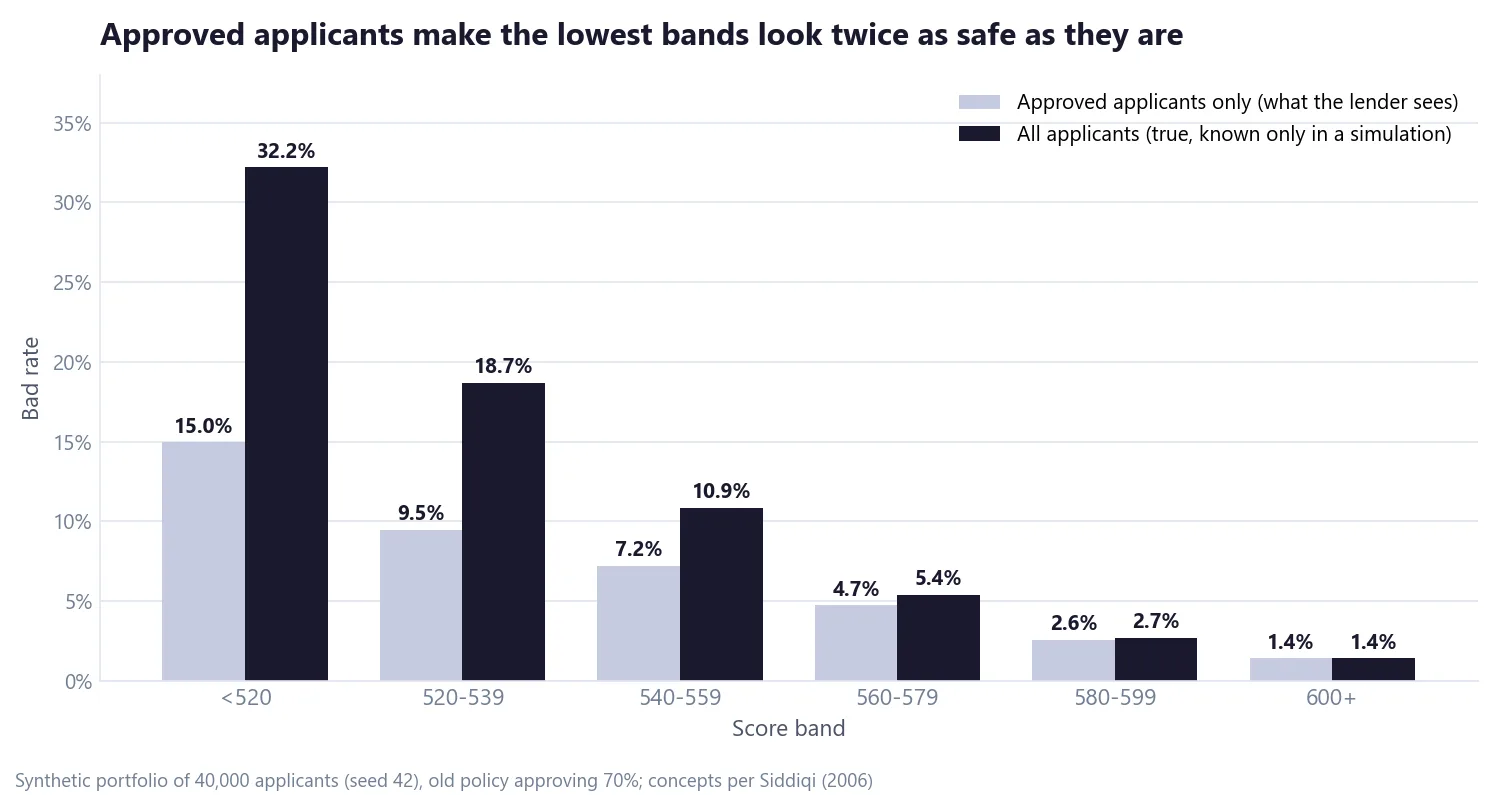
The gap is not spread evenly. Above 560 points the two bars nearly match, because the old policy approved most applicants there. Below 540 they split apart: 15% against 32% in the lowest band, and 9.5% against 18.7% in the next.
The reason is that applicants were declined for reasons the new model only partly captures. An underwriter saw something in the application, or the old scorecard used information the new one doesn't, and declined the riskier applicants within each band. The ones left behind look safer than the band really is.
This matters most exactly where it hurts. The cutoff, covered in Part 6, will sit in the lower bands. A model trained only on approved applicants will tell you those bands are much safer than they are, and the cutoff will be set too low.
Seven options for handling rejects
Reject inference assigns a likely outcome, good or bad, to applicants who were never approved, so they can join the development sample. The main techniques:
| Technique | How it works | Main weakness |
|---|---|---|
| Assign all rejects as bad | Every reject is counted as a bad | Overstates risk and repeats past decisions |
| Ignore rejects | Build on approved applicants only | Biased wherever past policy was selective |
| Approve a random sample | Approve some would-be rejects to observe them | Costly losses; slow to collect |
| Hard-cutoff augmentation | Score rejects with the approved-only model; below a chosen score call them bad, above it good | Depends on an arbitrary cutoff |
| Fuzzy augmentation | Split each reject into a weighted good and a weighted bad using its predicted probability | Assumes the approved-only model is right for rejects |
| Parcelling | In each score band, assign rejects as bad at the approved bad rate times a factor | The factor needs judgement or outside evidence |
| Bureau data | Use declined applicants' performance on similar credit obtained elsewhere | Needs bureau access within the rules; definitions may differ |
None of these is free. The first two are really ways of not doing reject inference. Random approval gives true answers, but it means knowingly lending to applicants you expect to lose money on, and Siddiqi notes it can also face legal hurdles in some jurisdictions (p. 104). The statistical methods all lean on the approved-only model being roughly right about the rejects, which is exactly what is in doubt.
Parcelling, band by band
Parcelling is a common middle ground, and it is easy to follow. In each score band:
inferred bads = number of rejects × approved bad rate × k
where k is a factor of 1 or more that rises as the score falls, because rejects are riskier than the approved applicants scored alongside them. The rest of the band's rejects are counted as goods, and the inferred accounts join the development sample alongside the known ones. The inferred bad rate for the band combines the approved bads and the inferred ones.
| Band | Approved | Rejects | Approved bad % | k | Inferred bads | Inferred bad % | True bad % |
|---|---|---|---|---|---|---|---|
| <520 | 274 | 2,357 | 15.0% | 1.6× | 564 | 23.0% | 32.2% |
| 520–539 | 2,148 | 4,036 | 9.5% | 1.5× | 575 | 12.6% | 18.7% |
| 540–559 | 7,464 | 4,166 | 7.2% | 1.4× | 421 | 8.3% | 10.9% |
| 560–579 | 9,209 | 1,333 | 4.7% | 1.3× | 82 | 4.9% | 5.4% |
| 580–599 | 6,525 | 108 | 2.6% | 1.2× | 3 | 2.6% | 2.7% |
| 600+ | 2,380 | 0 | 1.4% | 1.0× | 0 | 1.4% | 1.4% |
The table is calculated on unrounded bad rates. Take the lowest band: 2,357 rejects × 14.96% × 1.6 gives 564 inferred bads. Add the 41 bads among the 274 approved, divide by all 2,631 applicants in the band, and the inferred bad rate is 23.0%.
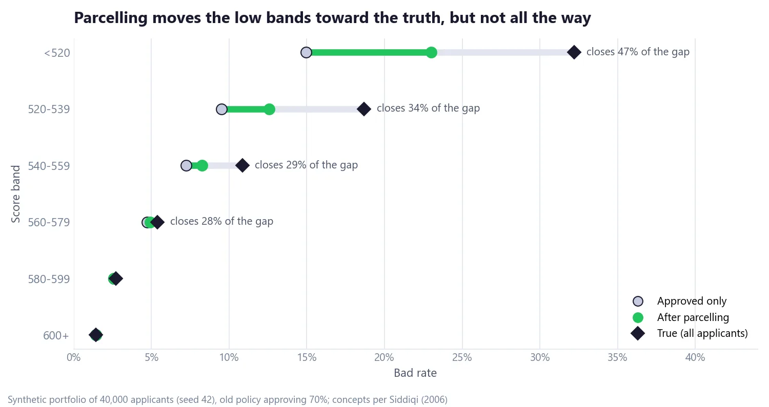
Parcelling moves every low band in the right direction, closing 28% to 47% of the gap across the four lowest bands. It does not close all of it, because the factor k here is a judgement call that turned out too low. That is the honest summary of most statistical reject inference: better than ignoring the rejects, but only as good as the assumption you feed it. In real data you never see the "true" column, so you can't check k against it. You need outside evidence.
Where a credit bureau comes in
That outside evidence is where credit bureaus come in. Siddiqi calls it the similar in-house or bureau data method: take applicants a lender declined who were approved for similar credit elsewhere, follow their repayment through credit bureau records, and use that as a proxy for how they would have performed (pp. 103–104). Short of actually approving them, it is the closest thing to observing the rejects directly.
This method is one of the things a credit bureau does best, and in my work at a credit bureau in Indonesia I see lenders use it. A bureau can match like with like: the same product type, the same type of financial institution, a similar time after the decline. That matching matters, because performance on a small personal loan says little about how someone would have handled a mortgage.
Two things make it harder than it sounds.
It is heavily regulated. Bureau data can't become a window into a competitor's book. Take OJK's own financial information service, SLIK, as an example. As of October 2026, a lender may use debtor information from SLIK only for permitted purposes, such as supporting lending decisions, managing credit risk, or meeting OJK's and other authorities' requirements on debtor quality. Every request has to be logged together with its purpose, and the regulator's official explanation allows prospect lists and cross-selling only on the lender's own customers (POJK 18/2017 as amended by POJK 11/2024, Article 15). Private credit bureaus are covered by a separate regulation, POJK 5/POJK.03/2022, under which the data a bureau collects may be used only to produce credit information (Article 46).
Siddiqi makes the same general point: regulatory hurdles may stop a creditor from obtaining bureau records of declined applicants, and where bureau data is strictly regulated the method may not be possible (p. 104). Any bureau-based reject inference study has to sit inside those rules.
The performance definition has to match. In my view, the best technique is the one that matches the performance definition the client actually uses, whether that is measured at application level, at bureau level across all of a borrower's credit, or on one product. Siddiqi flags the same issue: the bad definition chosen for the known goods and bads must be applied to the declined applicants' accounts elsewhere, using different data sources, "which may not be easily done" (p. 104). If declined applicants are labelled with the bureau's definition of bad instead of the lender's, the inferred bads measure a different thing from the known ones.
There is also a sample caveat. Applicants declined at one lender are likely to be declined elsewhere too, so the ones who did get credit are a selected and usually safer subset, and there may not be many of them.
Before you trust your inferred bads
A short checklist I would run on any reject inference result:
- Compare the approved-only and inferred bad rates band by band. If inference changed nothing in the low bands, it probably did nothing at all.
- Check that the inferred bad rate rises steadily as the score falls. A reversal means the factor or the model is off.
- Write down where every factor or cutoff came from. "Judgement" is an acceptable answer once; it should not be the only one.
- Look for outside evidence. Bureau performance on similar products, or a small random-approval test, is worth more than any statistical assumption.
- Match the performance definition. Outside evidence only counts if "bad" means the same thing in both places.
- Confirm the data use is permitted. Especially with bureau data, check the purpose is allowed and documented before the study starts, not after.
- Rebuild and compare. Fit the model with and without the inferred rejects, and look at how much the low-band points move.
Part 1 covered how points map to odds, Part 2 how "bad" is defined, and Part 3 how the model is fitted. Part 5 turns that model into a points table and measures how well it ranks risk, with KS, Gini and validation.
If you have run reject inference with bureau data, I would like to hear what you matched on: get in touch.
Hafizh Yuwan Fauzan (Hafizh Fauzan) is a credit risk data scientist in Jakarta, Indonesia, building scorecards and machine learning models on national-scale credit data.