Out-of-Time Validation for Credit Scorecards: OOT and Ultra OOT
By Hafizh Yuwan Fauzan · 2026-10-22
Stability deep dive 3 of 5: out-of-time and ultra OOT validation. The second deep dive looked at which characteristics moved; this one turns from applicants to outcomes.
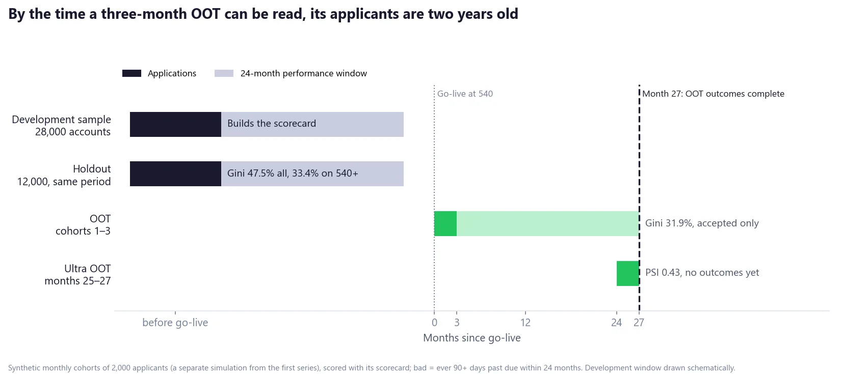
The out-of-time (OOT) Gini came back at 31.9%. The development report said 47.5%. A drop of 15.6 points looks like a scorecard that has stopped working.
It hasn't. The two numbers measure different populations. The 47.5% is the holdout Gini on every applicant. The 31.9% is on accounts the lender accepted, because only accepted accounts have outcomes. Measured on the holdout's own accepted accounts, the development benchmark is 33.4%, and the gap shrinks to 1.5 points, well inside the noise.
In my view this is the most common mistake in reading an OOT: the wrong benchmark. This deep dive is about the OOT done properly. It covers choosing the window, comparing like with like, what an OOT can and can't prove, and the ultra OOT check that covers the two years an OOT can't see.
The figures come from the same separate simulation as the earlier deep dives: monthly cohorts of 2,000 applicants for the fictional lender in Part 7 of the scorecard series, which went live at a 540 cutoff, scored with the scorecard from Part 5. Bad means ever 90+ days past due within 24 months. The development and holdout figures are the first series' own.
Out-of-sample is not out-of-time
A holdout is a random slice of the development data. Siddiqi recommends modelling on "a random 70% or 80% of the development sample" and keeping the rest as a "holdout sample" for validation (Credit Risk Scorecards, 2006, p. 127). That tests overfitting. It can't test time, because the holdout's applicants applied in the same months, under the same economy, marketing and policy, as the accounts the model learned from.
An OOT sample comes from a later period. Supervisors ask for both: the ECB's guide to internal models (July 2025 edition, since updated) says independent test data should cover "not only random sampling (out-of-sample), but also … different time periods (out-of-time) unless there are no sufficient data available" (ECB guide to internal models). As I wrote in Part 5, in my work an OOT is a must.
Choosing the window
Two rules decide where an OOT window can sit.
It must be mature. Every account needs its full performance window, or bads are still on their way. Siddiqi's example shows the size of the error: a sample opened seven months ago would show about 4.5% bad, against about 6% once mature, so "some accounts from this period that are bad would be erroneously labeled as good" (p. 35). With a 24-month bad definition, the youngest application in an OOT window is at least 24 months old on the day you read it.
It must be big enough. Gini on a few hundred bads is noisy.
I like a three-month window. A short window keeps the OOT as close to today as maturity allows. The price is sampling noise. For this lender, the first three cohorts after go-live give 4,697 accepted accounts and 339 bads. A bootstrap puts the standard error of their Gini at 2.6 points.
That noise is easy to see. Wait three more months for a six-month window (cohorts 1–6, readable at month 30) and the Gini is 35.9%, not 31.9%. It is the same scorecard, four points apart, and both are within two standard errors of the accepted holdout's 33.4%. A Gini that moves by two or three points between windows is not a change until it has been checked against the noise.
Compare like with like
| Sample | Accounts | Bads | Gini | Standard error | KS (at score) |
|---|---|---|---|---|---|
| Holdout, all applicants | 12,000 | 1,236 | 47.46% | – | 34.2% (545) |
| Holdout, accepted (540+) | 9,367 | 613 | 33.4% | 2.1 pts | 25.0% (560) |
| OOT, cohorts 1–3, accepted | 4,697 | 339 | 31.9% | 2.6 pts | 25.0% (570) |
| OOT, cohorts 1–6, accepted | 9,248 | 666 | 35.9% | 1.9 pts | 27.3% (560) |
Why does cutting off the declines take 14 points off the Gini? Gini measures how well the score separates goods from bads across its whole range. Below 540 sit the lowest scores and the densest bads. Remove them and what is left is a narrower range of scores, closer together, with fewer bads to find. The scorecard is the same; the job is harder.
After go-live there is no way around it: declined applicants never get a loan, so they never get an outcome. (That missing-outcome problem is the subject of Part 4 on reject inference.) The fix for the benchmark is simple. Apply the same cutoff to the holdout and recompute. Here, the OOT's 31.9% against 33.4% is a difference of 1.5 points, with a standard error of about 3.4 points on the difference. There is no evidence that the ranking has decayed. The level is a separate question, below.
The same applies to bad rates. The holdout's all-applicant bad rate is 10.3%; its accepted bad rate is 6.5%. Compare the OOT's accepted bad rate with the second, never the first.
What the OOT proves, and what it can't
An OOT can prove two things about the period it covers.
Rank order held. Bad rates by score band in the three-month OOT still fall steadily as scores rise:
| Score band | Accounts | Actual bad rate | Expected bad rate |
|---|---|---|---|
| 540–559 | 1,757 | 11.5% | 10.4% |
| 560–579 | 1,554 | 6.1% | 5.6% |
| 580–599 | 1,047 | 3.5% | 3.0% |
| 600+ | 339 | 1.5% | 1.5% |
Where the level stands. The expected bad rate comes from the scaling (600 points at 50 to 1, 20 points to double the odds). Overall, the OOT runs at 7.2% against 6.5% expected, about 11% above. Most of the gap sits in the 540–559 band, just above the cutoff; 600+ is on target. Part 7's first cohort showed the same kind of gap just above the cutoff, in a different simulation. Whether a gap like this grows, and what to do when it does, is the subject of the fifth deep dive.
What the OOT can't prove is anything about today. Look at what it was tested on. The score's monthly PSI in months 1 to 3 was 0.004 to 0.009: the OOT's applicants looked almost exactly like the development sample. The scorecard passed an easy exam. Siddiqi's warning about pre-implementation validation applies here too: "where the development sample is two or three years old, significant shifts in applicant profile may have occurred, and need to be identified" (p. 135).
On the day this OOT can first be read, month 27, its youngest applications are 24 months old. Whatever happened to applicants in those two years, the OOT doesn't know.
Siddiqi names the trap that follows, for a scorecard that fails validation: redeveloping "may not be a viable choice, since the data sample for this redevelopment will likely come from the same time period as the original scorecard, which did not validate" (p. 141). Outcomes will always lag. Stability is the only thing you can measure on recent applicants.
The ultra OOT: stability without outcomes
That is why, at the bureau where I work, we also run what we call an ultra OOT (Part 5 introduced it): the most recent applicants, too new to have any outcome, compared with the development sample on stability alone. It is the closest thing to the front-end validation in Siddiqi's pre-implementation step, which scores recent applications and compares their distributions with development (p. 136).
At month 27, the ultra OOT on months 25–27 reads:
| Months 25–27 vs development | Index |
|---|---|
| Score PSI | 0.43 |
| CSI, credit inquiries in the last 6 months | 0.49 |
| CSI, revolving utilisation | 0.38 |
| CSI, age | 0.22 |
| CSI, delinquencies, residential status, time at address | below 0.001 each |
The OOT says the scorecard ranked well on applicants from two years ago. The ultra OOT says today's applicants are far from the development sample. Both are true. They answer different questions, and neither answers the other's.
Two habits make the ultra OOT more useful.
Run it on several windows, not one. Siddiqi recommends running stability on "last month, last three months, last six months, and so on" to "detect any emerging trends, or to confirm that deviations in one particular month do not represent any long-term trend" (p. 136), and later: "identify trends, not quirks" (p. 163). The same check on months 16–18 read 0.14. Utilisation and age had been drifting for months, in the slow way the first deep dive traced. Something else arrived between month 18 and month 27.
Read every CSI next to the PSI, not after it. Inquiries are the largest single mover at 0.49, and that CSI wasn't there before: it went from 0.00 in month 19 to 0.47 in month 20, in one step. A real change in applicants rarely moves one characteristic that sharply on one date. Whether it is drift or a change in how the field is built is the question the next deep dive takes apart.
What the ultra OOT can't say is whether the shift matters for risk. A PSI of 0.43 tells you the population moved, not that the scorecard ranks worse on it. Siddiqi is careful on this point: similarity with development "while not conclusive, … provides a comfort level" (p. 164). The reverse holds too: a shift is a reason to investigate, not a verdict.
An OOT report card
This is the shape I would give an OOT and ultra OOT report, so the right numbers sit next to each other:
OOT window           cohorts, months of applications, date read (≥ performance window after the last one)
Size                 accounts, bads, Gini standard error (bootstrap)
Benchmark            holdout recomputed on the same cutoff, same bad definition
Discrimination       Gini and KS: OOT vs benchmark, difference vs its standard error
Rank order           bad rate by score band, actual vs expected
Level                actual ÷ expected bad rate, overall and by band
Ultra OOT            last 1, 3 and 6 months: score PSI and every CSI, no outcomes
Gap                  months between the OOT's youngest application and today
The last line is the easiest one to leave out. Everything above it describes the past, and the gap says how far in the past.
How long a window do you use for your OOT, and what do you compare it against? I would like to hear how others set it up. Get in touch.
Hafizh Yuwan Fauzan (Hafizh Fauzan) is a credit risk data scientist in Jakarta, Indonesia, building scorecards and machine learning models on national-scale credit data.